Creating Custom Legends

07 Oct 2020

Occasionally, the need might arise to generate your own custom legend for your data. I swear this happens often in the wild, but I’m pretty proud of how contrived an example I cooked up.

Example

Let’s say that we work for the Queenstown Ministry of Travel, that we have a naive understanding of causality, and that there’s a second Titanic ship coming into our port, which we know will sink.

Our job is to create the cleanest visualization to explain how our new legislation mandating that “all laborers (Male, third-class passengers) boarding in Queenstown must be between the ages 28 and 30” is for their own good.

We’ll start by loading up the Titanic data.

%pylab inline

from seaborn import load_dataset

df = load_dataset('titanic')

df.head(10)

Populating the interactive namespace from numpy and matplotlib

	survived	pclass	sex	age	sibsp	parch	fare	embarked	class	who	adult_male	deck	embark_town	alive	alone
0	0	3	male	22.0	1	0	7.2500	S	Third	man	True	NaN	Southampton	no	False
1	1	1	female	38.0	1	0	71.2833	C	First	woman	False	C	Cherbourg	yes	False
2	1	3	female	26.0	0	0	7.9250	S	Third	woman	False	NaN	Southampton	yes	True
3	1	1	female	35.0	1	0	53.1000	S	First	woman	False	C	Southampton	yes	False
4	0	3	male	35.0	0	0	8.0500	S	Third	man	True	NaN	Southampton	no	True
5	0	3	male	NaN	0	0	8.4583	Q	Third	man	True	NaN	Queenstown	no	True
6	0	1	male	54.0	0	0	51.8625	S	First	man	True	E	Southampton	no	True
7	0	3	male	2.0	3	1	21.0750	S	Third	child	False	NaN	Southampton	no	False
8	1	3	female	27.0	0	2	11.1333	S	Third	woman	False	NaN	Southampton	yes	False
9	1	2	female	14.0	1	0	30.0708	C	Second	child	False	NaN	Cherbourg	yes	False

Then create a new feature, derived from a combination of sex, embark location, and the passenger class.

Inspecting, there are 18 different combinations of these three features.

df['sex_embark_class'] = df['sex'] + ' ' + df['embarked'] + ' ' + df['pclass'].astype(str)

df['sex_embark_class'].nunique()

Due to our shoddy understanding of statistics, the only things we care about communicating are the relationship between:

Age
Sex + Board Location + Class
Mortality

As we’re sufficiently convinced that these are all the features we need to make an accurate prediction when history repeats itself.

Plotting death by age, separated by sex_embark_class, we immediately stumble into a busy, uninformative graph.

fig, ax = plt.subplots(figsize=(14, 5))

for idx, group in df.groupby('sex_embark_class'):
    ax.scatter(group['age'], group['survived'], alpha=.5, label=idx, s=20)
    
ax.set_xlabel('age')
ax.set_ylabel('death')
ax.legend();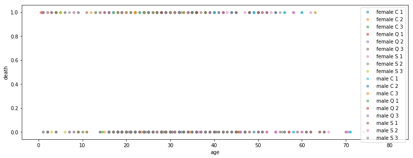

png

Cleaning up a bit, we might generate a couple dictionaries to help us conditionally-color/size the markers, based on if they’re in our target pop.

However, there’s still the matter of the busy legend– we don’t care what all the other markers are. We’re trying to separate this problem into a simple binary classification problem.

fig, ax = plt.subplots(figsize=(14, 5))

color_dict = {True: 'orange', False: 'grey'}
size_dict = {True: 40, False: 10}

for idx, group in df.groupby('sex_embark_class'):
    is_queenstown_laborer = (idx == 'male Q 3')
    ax.scatter(group['age'],
               group['survived'],
               alpha=.5,
               label=idx,
               s=size_dict[is_queenstown_laborer],
               c=color_dict[is_queenstown_laborer])
    
ax.set_xlabel('age')
ax.set_ylabel('death')    
ax.legend();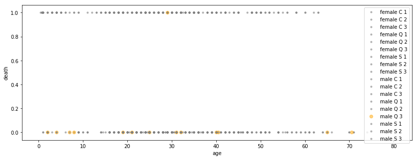

png

Shit. Changing the label didn’t work.

fig, ax = plt.subplots(figsize=(14, 5))

color_dict = {True: 'orange', False: 'grey'}
size_dict = {True: 40, False: 10}

for idx, group in df.groupby('sex_embark_class'):
    is_queenstown_laborer = (idx == 'male Q 3')
    ax.scatter(group['age'],
               group['survived'],
               alpha=.5,
               label=str(is_queenstown_laborer),
               s=size_dict[is_queenstown_laborer],
               c=color_dict[is_queenstown_laborer])
    
ax.set_xlabel('age')
ax.set_ylabel('death')    
ax.legend();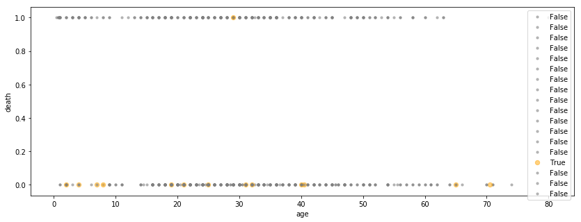

png

The Point of this Notebook

Finally, we arrive at the motivation for this tutorial: The legend that gets generated for us is too busy, and we’re not particularly interested in rewriting our DataFrame code to include a new field, just for the sake of vizualization.

Instead, we can use matplotlib.patches.Rectangle objects (docs) like so

from matplotlib.patches import Rectangle

handles = [
    Rectangle((0, 0), 1, 1, color='orange'),
    Rectangle((0, 0), 1, 1, color='gray')    
]
labels = ['You', 'Not You']

Then, the main differences in our code are tossing the label=idx in the ax.scatter() call, and passing in handles and labels generated above.

I added the axvlines for more clarity.

fig, ax = plt.subplots(figsize=(14, 5))

color_dict = {True: 'orange', False: 'grey'}
size_dict = {True: 40, False: 10}

for idx, group in df.groupby('sex_embark_class'):
    is_queenstown_laborer = (idx == 'male Q 3')
    ax.scatter(group['age'],
               group['survived'],
               alpha=.5,
               s=size_dict[is_queenstown_laborer],
               c=color_dict[is_queenstown_laborer])

ax.axvline(28, c='r', alpha=.5)
ax.axvline(30, c='r', alpha=.5)
ax.legend(handles, labels, loc='right');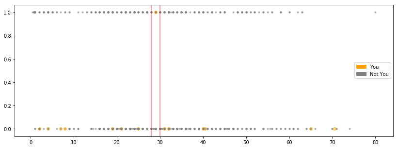

png

Looking at that last call to ax.legend(), it’s obvious to me what labels and loc mean. However, handles is less clear.

Reading up on it, it just looks like the terminology is just a legacy decision that’s worth remembering, because it’s part of the vocabulary of the whole design of the legend feature.