F Statistic
Overview
The F-Statistic of a Linear Regression seeks to answer “Does the introduction of these variables give us greater information gain when trying to explain variation in our target?”
I like the way that Ben Lambert explains and will paraphrase.
First you make two models– a restricted model that’s just the intercept and an unrestricted model that includes new x_i values
$R: y = \alpha $
$U: y = \alpha + \beta_1 x_1 + \beta_2 x_2$
Then our Null Hypothesis states that none of the coefficients in U matter and B_1 = B_2 = 0 (but can extend to arbitrarily-many Beta values). Equivalently, the alternative hypothesis states that B_i != 0 for either Beta.
And so we start by calculating the Sum of Squared Residuals (see notes on R-Squared for refresher) for both the Restricted and Unrestricted models.
By definition, then SSR for the Restricted will be higher– addition of any X variables will account for some increase in predictive power even if miniscule.
Armed with these two, the F-Statistic is simply the ratio of explained variance and unexplained variance, and is calculated as
$F = \frac{SSR_R - SSR_U}{SSR_U}$
Well, almost.
We also, critically, normalize the numerator and denominator based on p, the number of x features we’re looking at, and n, the number of observations we have. This helps us account for degrees of freedom and looks like the following:
$F = \frac{(SSR_R - SSR_U)/p}{SSR_U/(n-p-1)}$
Interpretation
Plugging this into your favorite statistical computing software will yield a value that can take on wildly-different values. Conceptually, let’s imagine two extremes:
- The X values don’t give us anything useful. This means that the numerator (the information gain of adding them to the model) is small, therefore the whole fraction is small (often around
1or so) - On the other hand, if there’s a huge improvement, you might see F values in the hundreds, if not thousands.
Generally, the F-statistic follows a distribution that depends on the degrees of freedom for both the numerator and denominator, and has a shape that looks like the following.
from IPython.display import Image
Image('images/f_dists.PNG')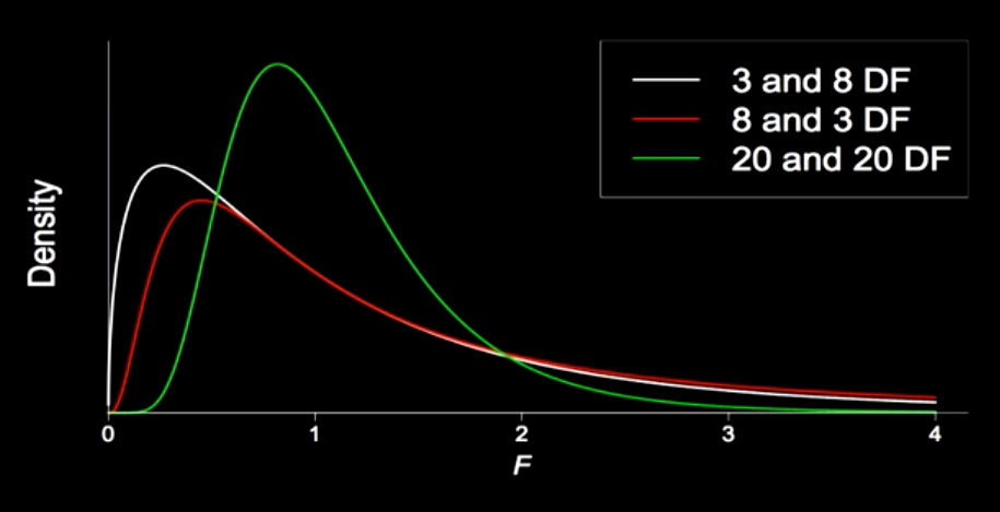
Relationship to t-statistic
The F and t statistics feel conceptually adjacent. But whereas F examines the effect of multiple attributes on your model, the t simply looks at one.
From a notation standpoint, if you had a model with an intercept and one x and wanted to observe the F statistic when introducing another x, you’d have a difference in 1 degree of freedom (numerator), and 2 degrees of freedom (minus the standard 1 in the denominator), thus
$F_{1, N-3}$
As far as the output goes, this is functionally equivalent to finding the t-statistic for the same degrees of freedom (N-3), and squaring it. Source
An Example
If we whip up a quick Linear Regression using the statsmodels.api and the boston dataset within sklearn, we get access to a very clean object that we can use to interrogate the F-statistic for the model as a whole
import statsmodels.api as sm
from sklearn.datasets import load_boston

data = load_boston()

X = data['data']
X = sm.add_constant(X)

est = sm.OLS(data['target'], X)
est = est.fit()

est.fvalue
108.07666617432622
But we also can see, using .summary(), the t-statistic for each of the attributes of our model. This is the same as omitting the variable, calculating the F-statistic, then taking the square root (and changing the sign, where appropriate).
In other words, this is the same as the partial effect of adding this variable to the mix.
est.summary()| Dep. Variable: | y | R-squared: | 0.741 |
|---|---|---|---|
| Model: | OLS | Adj. R-squared: | 0.734 |
| Method: | Least Squares | F-statistic: | 108.1 |
| Date: | Mon, 09 Sep 2019 | Prob (F-statistic): | 6.72e-135 |
| Time: | 16:44:05 | Log-Likelihood: | -1498.8 |
| No. Observations: | 506 | AIC: | 3026. |
| Df Residuals: | 492 | BIC: | 3085. |
| Df Model: | 13 | ||
| Covariance Type: | nonrobust |
| coef | std err | t | P>|t| | [0.025 | 0.975] | |
|---|---|---|---|---|---|---|
| const | 36.4595 | 5.103 | 7.144 | 0.000 | 26.432 | 46.487 |
| x1 | -0.1080 | 0.033 | -3.287 | 0.001 | -0.173 | -0.043 |
| x2 | 0.0464 | 0.014 | 3.382 | 0.001 | 0.019 | 0.073 |
| x3 | 0.0206 | 0.061 | 0.334 | 0.738 | -0.100 | 0.141 |
| x4 | 2.6867 | 0.862 | 3.118 | 0.002 | 0.994 | 4.380 |
| x5 | -17.7666 | 3.820 | -4.651 | 0.000 | -25.272 | -10.262 |
| x6 | 3.8099 | 0.418 | 9.116 | 0.000 | 2.989 | 4.631 |
| x7 | 0.0007 | 0.013 | 0.052 | 0.958 | -0.025 | 0.027 |
| x8 | -1.4756 | 0.199 | -7.398 | 0.000 | -1.867 | -1.084 |
| x9 | 0.3060 | 0.066 | 4.613 | 0.000 | 0.176 | 0.436 |
| x10 | -0.0123 | 0.004 | -3.280 | 0.001 | -0.020 | -0.005 |
| x11 | -0.9527 | 0.131 | -7.283 | 0.000 | -1.210 | -0.696 |
| x12 | 0.0093 | 0.003 | 3.467 | 0.001 | 0.004 | 0.015 |
| x13 | -0.5248 | 0.051 | -10.347 | 0.000 | -0.624 | -0.425 |
| Omnibus: | 178.041 | Durbin-Watson: | 1.078 |
|---|---|---|---|
| Prob(Omnibus): | 0.000 | Jarque-Bera (JB): | 783.126 |
| Skew: | 1.521 | Prob(JB): | 8.84e-171 |
| Kurtosis: | 8.281 | Cond. No. | 1.51e+04 |
Warnings:
[1] Standard Errors assume that the covariance matrix of the errors is correctly specified.
[2] The condition number is large, 1.51e+04. This might indicate that there are
strong multicollinearity or other numerical problems.
A warning about .summary() method and t-statistics
It’s not enough to consider all of the t-statistics for each coefficient.
Consider the case when we build a Linear Regression off of 100 different attributes and that our null hypothesis is true– each of them are unrelated to the target.
Recall that the p-value is shorthood for “probability that we observed this statistic under the null hypothesis.” We often reject values less than 0.05, but considering the joint probability of 100 attributes, it’s likely that we incidentally see one of them coming in under this cutoff– despite not being valid.
If our criteria for “is this model valid?” is throwing a big ol’ OR statement on all of the p-values and hoping for a bite, we’re likely to come to a false conclusion.
On the other hand, looking at the F statistic, because of the normalization by n and p, accounts for the observation and dimension size.