Forward Propagation

Forward propogation in a Neural Network is just an extrapolation of how we worked with Logistic Regression, where the caluculation chain just looked like

from IPython.display import Image

Image('images/logit.PNG')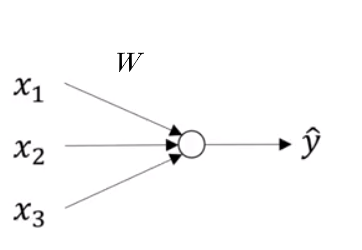

Our equation before,

$\hat{y} = w^{T} X + b$

was much simpler in the sense that:

• X was an n x m vector (n features, m training examples)
• This was matrix-multiplied by w an n x 1 vector of weights (n because we want a weight per feature)
• Then we broadcast-added b
• Until we wound up with an m x 1 vector of predictions

A Different Curse of Dimensionality

Now when we get into Neural Networks, with multiple-dimension matrix-multiplication to go from layer to layer, things can get pretty hairy.

Image('images/dimensions.PNG')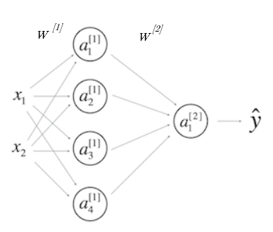

Terminology

• Our input layer X is still n x m
• Our output layer is still m x 1.
• Hidden/Activation layers are the nodes organized vertically that represent intermediate calculations.
  • The superscript represents which layer a node falls in
  • The subscript is which particular node you’re referencing
• The weights matricies are the values that take you from one layer to the next via matrix multiplication.
  • *PAY CAREFUL ATTENTION TO THE FACT that W1 takes you from layer 1 to layer 2*

Keeping the Dimensions Straight

Always refer back to the fact that dot-producting two matricies along a central dimension cancels it out. For instance:

Image('images/cancelling.png')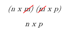

Therefore, understanding which dimension your data should be in is an exercise in plugging all of the gaps to get you from X to y

W1

Getting to a2 means following the equation

$a^{[2]} = W^{[1]}X$

As far as dimensions go, we’re looking at

• X: n x m
• a1: 4 x m

Subbing the dimensions in for the variables, we can start to fill in the gaps

$(4, m) = (?, ??) (n, m)$

because we know that we want 4 as the first value

$(4, m) = (4, ??) (n, m)$

we just need

$(4, m) = (4, n) (n, m)$

Thus

$dim_{W} = (4, n)$

More Generally

If layer j is m-dimensional and layer j+1 is n-dimensional

$W^{j} \quad \text{(which maps from j to j+1) has dimensionality} \quad (n \times m)$

Vectorizing the Implementation

The following image (grabbed from Computing a Neural Network’s Output in Week 3) is as busy as it is informative.

It color-codes the same simple as above, highlighting the stacking approach to go from various vectors (e.g. z[1]1, z[1]2, z[1]3, z[1]4) to one large, unified matrix of values (Z[1])

Image('images/vectorizing.png')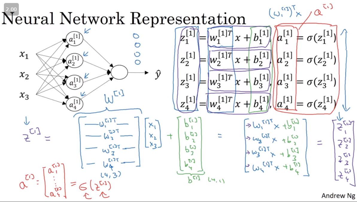

And so the process becomes 4 simple equations for one training example

$z^{[1]} = W^{[1]} x + b^{[1]}$

$a^{[1]} = sigmoid(z^{[1]})$

$z^{[2]} = W^{[2]} a^{[1]} + b^{[2]}$

$a^{[2]} = sigmoid(z^{[2]})$

In Python

z1 = np.dot(W1, x) + b1
a1 = sigmoid(z1)
z2 = np.dot(W2, a1) + b2
a2 = sigmoid(z2)

If you want to extend to multiple training examples, you introduce a (i) notation, where

$a_{2}^{1}$

refers to the 2nd node activation, in the 1st hidden layer, of the ith training example. And propogating for each prediction involves a big for loop

for i in range(len(x)):
    z1[i] = np.dot(W1, x[i]) + b1
    a1[i] = sigmoid(z1[i])
    z2[i] = np.dot(W2, a1[i]) + b2
    a2[i] = sigmoid(z2[i])

Or less-awfully, we can vectorize the whole thing

$Z^{[1]} = W^{[1]}X + b^{[1]}$

$A^{[1]} = sigmoid(Z^{[1]})$

$Z^{[2]} = W^{[2]}A^{1} + b^{[2]}$

$A^{[2]} = sigmoid(Z^{[2]})$

In Python

Z1 = np.dot(W1, X) + b1
A1 = sigmoid(Z1)
Z2 = np.dot(W2, A1) + b2
A2 = sigmoid(Z2)