Residual Networks

Motivation

Consider a very deep image-classification neural network like the one below

from IPython.display import Image

Image('images/very_deep_network.png')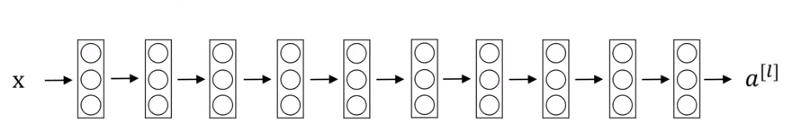

A typical shortcoming of this sort of architecture is overfitting of the data.

This is a result of information gain from back-propagation not making it all the way back to our earlier layers in the network (due to the vanishing gradient problem). After a certain point, the earlier layers stop changing much at all, and the later layers over-adjust to the data it’s trained on.

Residual Networks provide an approach to take us from error-over-train-time on the left to on the right.

Image('images/resnet_error.png')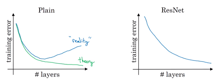

Skip Connections

It does this by constructing “Shot Cut” or “Skip connections” like the ones below.

Image('images/very_deep_resnet.png')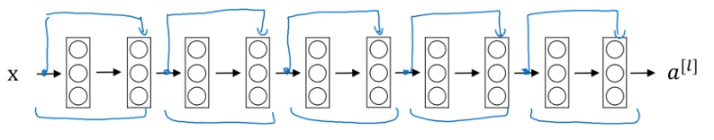

In a typical network, we go from a_L to a_L2 using the following.

$ a^{L} $

$ z^{L+1} = W^{L+1}a^{L} + b^{L+1} $

$ a^{L+1} = g(Z^{L+1}) $

$ z^{L+2} = W^{L+2}a^{L+1} + b^{L+2} $

$ a^{L+2} = g(Z^{L+2}) $

The key difference in a Residual Network is a revision of the last step to include a connection from a previous layer before application of the activation function.

$a^{L+2} = g(Z^{L+2} + a^{L})$

This allows us to both:

• Pass initial information deeper into the network
• Update our earlier weights more effectively

Why this Works

The intuition of why this helps is a bit hard to unpack, but if you can convince yourself that you’re, at the very least, able to have performance as good as a regular NN, then it makes enough sense that having more training parameters can only help improve the feature-richness of your model.

Identity Function

If we go from A to C by passing through B and find that A and C are exactly the same, then we consider B to be the identity function

Similarly if we look at the final equal equation for a_L2 above, we’ll see that it’s a function of Z_L2 and a_L. However, if the model learns that the appropriate weights and biases for Z_L1 are just 0, then we’re right back where we started with our value a_L.

Image('images/resnet_intuition.png')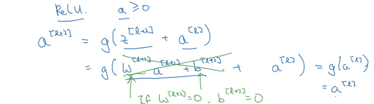

Dimensionality

It’s important to note that in order for this to work correctly, you must ensure that your shortcut calculations are operating over data of the exact same dimensions.

That’s to say that in this example, we can do whatever convolution/intermediate calculations we want between a_L and a_L2 as long as the dimension of the two are the same in the end.

Different ResNet Blocks

Identity Block

As we’ve stated before, the skip connection can skip over arbitrarily-many transformations, provided that the end result matches the dimensions of the layer we intend to use as a skip layer.

Image('images/resnet_arbitrary.png')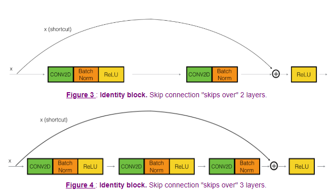

Convolution Block

Similarly, we can construct convolution blocks that follow the same idea with the slight variation that our final layer should have the same dimensions as our input, with some convolution applied.

Image('images/conv_block.png')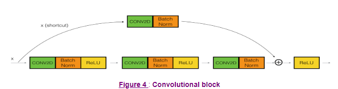

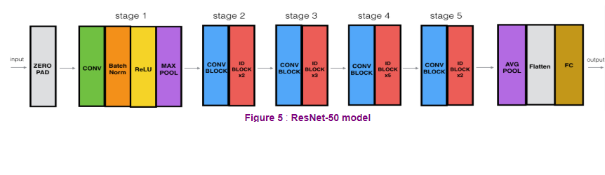
ResNet 50

Thus at scale, we can relatively-cheaply construct some robust networks.

Each intermediate stage opens with a Convolution Block that reduces the dimensionality from one stage to the next, then arbitrarily-many Identity Blocks to extract more complicated features.

Image('images/resnet_50.png')