Assortativity

04 Mar 2021

When examining the nature of your network’s arrangement, the concept of assortativity is a complicated, albeit deeply-intuitive one. You can think of it as the network analog to a correlation or coincidence score– it’s bounded between [-1, 1] and represents how much nodes in the network have self-arranged with other nodes that look like it.

Data

To dive into this concept, I’ll borrow a dataset representing faculty relationships at a university, keyed by the department they work in (group for each node).

(Link)

%pylab inline

import networkx as nx

G = nx.read_graphml('data/univ_dataset_TSPE.graphml')

Populating the interactive namespace from numpy and matplotlib

# simple helper function

pos = None

def draw(G, new_pos=False, colors=None):
    global pos
    
    if (pos is None) or new_pos:
        pos = nx.spring_layout(G)
        
    fig, ax = plt.subplots(figsize=(20, 10))
    nx.draw(G, alpha=.5, pos=pos, node_color=colors)

Inexplicably, every time I run it, there’s this wild outlier

draw(G)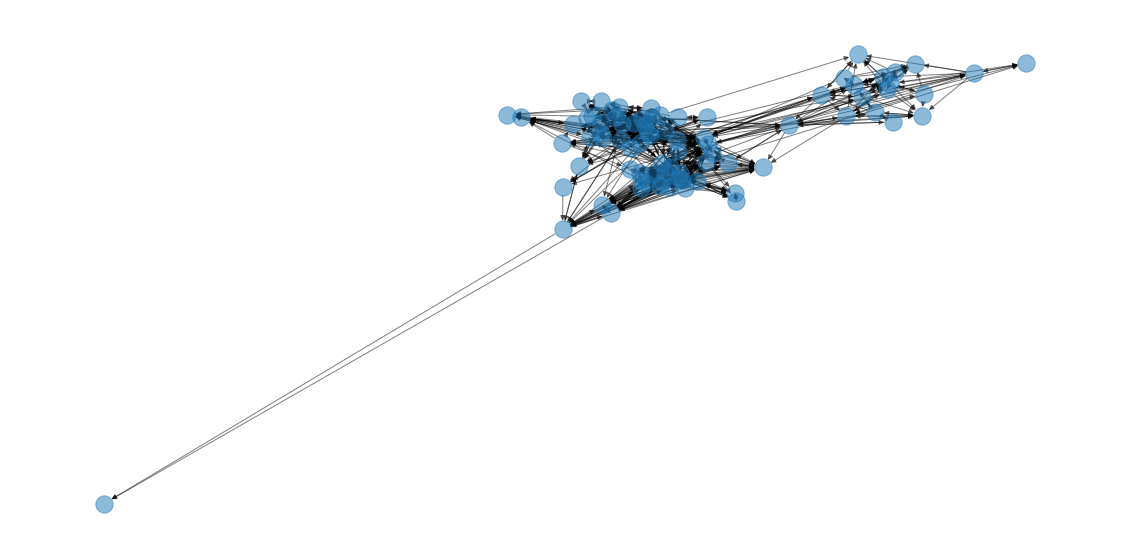

png

so I’m going to drop it for the sake of visual clarity.

G.remove_node('n10')

Much better!

Now to the matter at hand. How much did this network self-organize by the node attribute group?

group_dict = {idx: node['group'] for idx, node in G.nodes(data=True)}

color_dict = {0.0: 'red',
              1.0: 'blue',
              2.0: 'green',
              3.0: 'black'}

colors = [color_dict[group] for group in group_dict.values()]

A fair amount, it seems

draw(G, new_pos=True, colors=colors)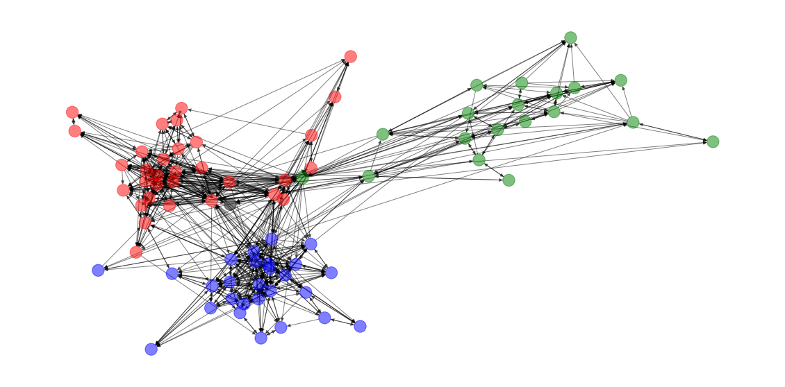

png

In fact, the assortativity coefficient is actually quite high.

nx.attribute_assortativity_coefficient(G, 'group')

0.7048747599784635

… but how did we arrive at it?

Constituent Parts

Before we walk through the underlying networkx code, I want to share the key formula from the seminal paper on the topic.

The following equation gives us the assortativity coefficient, r. Here, we’re only considering the discrete case (continuous in a few)– the paper that introduces the concept starts by encoding a categorical variable to numeric and going from there.

from IPython.display import Image

Image('images/assortativity.png')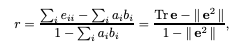

png

Let’s break this down a bit, using the table they provided at the beginning

r represents the assortativity coefficient
e is the “fraction of edges in a network that connect a vertex of type i to type j”. This is essentially a co-incidence matrix, normalized by the number of values, therefore the value of e sum to 1.

e = np.array([[.258, .016, .035, .013],
              [.012, .157, .058, .019],
              [.013, .023, .306, .035],
              [.005, .007, .024, .016]])

sum(e)

0.9969999999999999

For a given node, i, the a and b terms are the fraction of that node’s in/outbound edges that connect to the various other classes. In an undirected graph, these are equivalent.

a = np.sum(e, axis=1)
b = np.sum(e, axis=0)

display(a)
display(b)

array([0.322, 0.246, 0.377, 0.052])



array([0.288, 0.203, 0.423, 0.083])

Tr is a Linear Algebra operation where you sum the values along the diag. So in the right-hand chunk, summing e down the diag means summing the total proportion of edges in the network that map from same-type to same-type nodes.

tr_e = np.trace(e)
tr_e

0.7370000000000001

The double-bar e**2 term is a bit dense. Double-bar in this context means “the sum of all elements in the matrix”, that’s easy enough. Otherwise, you should recognize that squaring the matrix e and taking the sum of a * b for all values of i are literally the same thing– just consolidates it all into one step.

Stare at this until you believe that.

np.sum(a * b)

0.30646100000000004

e_squared_barbar = np.sum(e @ e)
e_squared_barbar

0.306461

Putting it altogether, we get

(
    (tr_e - e_squared_barbar)
    /
    (1 - e_squared_barbar)
)

0.6207855650511365

which is consistent with the value reported in the paper.

Image('images/assortativity.png')

png

In `networkx`

Getting back to it, let’s see how this is all stitched together under the hood.

node_attribute_xy

In the example above, we started with our matrix, e– the proportional coincidence matrix. So before we can really get going, we have to start there.

The nx.node_attribute_xy() function is an awesome generator that looks at every edge to serve up the attribute tuple for each connected pair

xy = list(nx.node_attribute_xy(G, attribute='group'))

list(
    (a, b)
    for (a, b) in xy
    if a != b
)[:10]

[(1.0, 0.0),
 (1.0, 0.0),
 (1.0, 0.0),
 (1.0, 2.0),
 (1.0, 2.0),
 (1.0, 2.0),
 (1.0, 3.0),
 (1.0, 0.0),
 (1.0, 0.0),
 (1.0, 3.0)]

mixing_dict

Next, we pipe that list of tuples into nx.mixing_dict() to get a nested-dict representation of our matrix e

nx.mixing_dict(xy)

{2.0: {2.0: 96, 0.0: 21, 1.0: 13, 3.0: 2},
 0.0: {0.0: 315, 1.0: 41, 3.0: 14, 2.0: 13},
 1.0: {0.0: 24, 1.0: 250, 2.0: 6, 3.0: 2},
 3.0: {0.0: 11, 3.0: 2, 2.0: 2, 1.0: 3}}

Alternatively, we could just use the following function that combines the last two steps

mixing_dict = nx.attribute_mixing_dict(G, 'group')

mixing_matrix

Finally, we build our e matrix from the mixing dict, calculated above.

manual = np.zeros((4, 4))

for i, row in enumerate(sorted(mixing_dict)):
    for j, col in enumerate(sorted(mixing_dict[row])):
        manual[i][j] = mixing_dict[row][col]
        
manual

array([[315.,  41.,  13.,  14.],
       [ 24., 250.,   6.,   2.],
       [ 21.,  13.,  96.,   2.],
       [ 11.,   3.,   2.,   2.]])

Of course, there’s a simple helper method that does this for us.

We can either get this as raw counts

mix_mat_raw = nx.attribute_mixing_matrix(G, 'group', normalized=False)
mix_mat_raw

array([[315.,  41.,  13.,  14.],
       [ 24., 250.,   6.,   2.],
       [ 21.,  13.,  96.,   2.],
       [ 11.,   3.,   2.,   2.]])

Or normalize the whole thing to sum to 1 (which is a necessary characteristic of e)

mix_mat_raw / mix_mat_raw.sum()

array([[0.38650307, 0.05030675, 0.01595092, 0.01717791],
       [0.02944785, 0.30674847, 0.00736196, 0.00245399],
       [0.02576687, 0.01595092, 0.11779141, 0.00245399],
       [0.01349693, 0.00368098, 0.00245399, 0.00245399]])

mix_mat = nx.attribute_mixing_matrix(G, 'group')
mix_mat

array([[0.38650307, 0.05030675, 0.01595092, 0.01717791],
       [0.02944785, 0.30674847, 0.00736196, 0.00245399],
       [0.02576687, 0.01595092, 0.11779141, 0.00245399],
       [0.01349693, 0.00368098, 0.00245399, 0.00245399]])

Finally, we plug-and-chug as above and see a considerable assortativity by group– which mirrors our visual intuition nicely

tr_e = mix_mat.trace()

e_squared_barbar = np.sum(mix_mat @ mix_mat)

(
    (tr_e - e_squared_barbar)
    /
    (1 - e_squared_barbar)
)

0.7048747599784635

In the likely event that you don’t want to do this all by hand, there’s absolutely a function that handles this all in a flash.

nx.attribute_assortativity_coefficient(G, 'group')

0.7048747599784635

Continuous Analog

Although the actual math is different, it’s possible to run the same function to apply the same general method on arbitrary continuous data.

To demonstrate, let’s build a trivial variable, based on the id value that a node gets instantiated with.

list((
    data
    for    node, data
    in     G.nodes(data=True)
))[:5]

[{'group': 2.0, 'id': 'n0'},
 {'group': 0.0, 'id': 'n1'},
 {'group': 2.0, 'id': 'n2'},
 {'group': 2.0, 'id': 'n3'},
 {'group': 1.0, 'id': 'n4'}]

Literally, just stripping off the leading n and casting as an int

node_ids = {node: int(data['id'][1:])
             for node, data 
             in G.nodes(data=True)}

nx.set_node_attributes(G, values=node_ids, name='node_id')

list((
    data
    for    node, data
    in     G.nodes(data=True)
))[:5]

[{'group': 2.0, 'id': 'n0', 'node_id': 0},
 {'group': 0.0, 'id': 'n1', 'node_id': 1},
 {'group': 2.0, 'id': 'n2', 'node_id': 2},
 {'group': 2.0, 'id': 'n3', 'node_id': 3},
 {'group': 1.0, 'id': 'n4', 'node_id': 4}]

And so running the equation over our node_id values, we get a value that’s very close to 0, suggesting that there is NO assortativity, with respect to node_id.

Put another way, this suggests that the nodes were introduced to the network in a random fashion– as we showed above there is clearly assortativity by group. So if nodes were added one group at a time, it follows that there would be a high degree of intra-group correlation. Summing that over the network, we’d expect to see something positive but small, probably in the .2-.4 range.

nx.attribute_assortativity_coefficient(G, 'node_id')

-0.015185949939552698

Degree Assortativity

Finally, we can peek at one of the more popular measures in this space and see how degree assortative our data is.

Do high-degree nodes disproportionately seek out other high degree nodes? Think about it: how often do celebrities marry total nobodies, vs other “nodes” with comparable star power?

To start, we’ll tack on a raw degree attribute and calculate the way we know how.

degrees = {node: degree
             for node, degree 
             in G.degree}

nx.set_node_attributes(G, values=degrees, name='degree')

list((
    data
    for    node, data
    in     G.nodes(data=True)
))[:5]

[{'group': 2.0, 'id': 'n0', 'node_id': 0, 'degree': 15},
 {'group': 0.0, 'id': 'n1', 'node_id': 1, 'degree': 36},
 {'group': 2.0, 'id': 'n2', 'node_id': 2, 'degree': 8},
 {'group': 2.0, 'id': 'n3', 'node_id': 3, 'degree': 18},
 {'group': 1.0, 'id': 'n4', 'node_id': 4, 'degree': 38}]

Looks pretty random to me.

nx.attribute_assortativity_coefficient(G, 'degree')

-0.0015635016182241753

Checking against the native function, I was surprised by how much I was off

nx.degree_assortativity_coefficient(G)

0.0356095440281665

Until I realized that this particular network is a directed graph

type(G)

networkx.classes.digraph.DiGraph

And that there’s an additional wrinkle you have to keep straight when rewriting the equation for r to consider in-degree vs out-degree separately. I’ll omit the particulars for now, but if it turns out that this is crucial to understand, I’ll come back and elaborate.

Casting G as an undirected graph for a sec, this is MUCH closer to what we did more manually :)

nx.degree_assortativity_coefficient(nx.Graph(G))

-0.004034673332927811